Code
library(tidyverse)
library(tidymodels)
library(gt)

set.seed(1234)

require(doParallel)
cores <- parallel::detectCores(logical = FALSE)I do not know a lot about college basketball. I follow the travails of my employer and a little about the Big Ten Conference as a whole, but at best it’s surface knowledge. I kinda know who is good that we’re going to play and who isn’t. Beyond that, nada.
Which is bad when it comes to tournament time.
My typical pattern of filling out bracket is Have I Heard Of This Team, Do They Have a Legendary Coach or Do I Hate Them For Some Reason. Depending on the answers, I make my pick. It’s not rocket science, and it rarely works.
This season, along with my SPMC460 Advanced Sports Data Analysis class, I decided to try use machine learning to get me a better bracket. The class is about the use of machine learning in sports, and so we’re going to use classification algorithms to decide a simple W or L designation.
What follows is the logic and the code I used to fill out my bracket.
How did it go?
Not great. Could I have done better guessing? Doubtful.
What I’m using to make and feed the model is the Tidyverse and Tidymodels set of libraries, the gt library for presenting some tables later, and doParallel for parallel processing, because the xgboost model training takes a while.
library(tidyverse)
library(tidymodels)
library(gt)
set.seed(1234)
require(doParallel)
cores <- parallel::detectCores(logical = FALSE)The data I’m using is scraped from Sports Reference and it’s the box scores of every Division I college basketball game since the start of the 2014-2015 season. The data is a little funny in that each game is in there twice – I’m scraping school pages, so the Team is always that school, and the Opponent is someone else. So a game between two Division I schools will appear twice – one for each Team.
My logic in picking predictors was that how efficient teams are with the ball is important, so I estimated the number of possessions and then calculated offensive and defensive ratings (which is points per 100 possessions).
I then wanted some kind of a metric of how good of a win or how bad of a loss a particular game was. So I calculated the score margin and added it to the opponent’s simple rating from Sports Reference. So a team losing close to a good team isn’t a bad loss. A bad team beating a good team is a great win. And so on. So if you’re a team beating up on bad teams, you don’t get a lot of credit for that.
Then, I used the teams cumulative mean over the course of the season to estimate what they would have going into the game. Obviously, you can’t know how a team will play going into a game, but I figure that they’ll be somewhere around their cumulative mean, which should pick up if the team is playing better or worse over a few games.
Then, for tournament purposes, I cut that to the last 10 games of the season. You are who you are in your last 10 games before the end of the season.
At least, that was my thinking.
games <- read_csv("http://mattwaite.github.io/sportsdatafiles/cbblogs1521.csv") %>% mutate(
  Possessions = .5*(TeamFGA - TeamOffRebounds + TeamTurnovers + (.475 * TeamFTA)) + .5*(OpponentFGA - OpponentOffRebounds + OpponentTurnovers + (.475 * OpponentFTA)),
  OffensiveRating = (TeamScore/Possessions)*100,
  DefensiveRating = (OpponentScore/Possessions)*100,
  ScoreDifference = TeamScore - OpponentScore,
  WinQuality = case_when(is.na(OpponentSRS) == TRUE ~ ScoreDifference, TRUE ~ ScoreDifference + OpponentSRS)
  ) %>%
  group_by(Team, Season) %>%
  mutate(
  Cumulative_Mean_Offensive = cummean(OffensiveRating),
  Cumulative_Mean_Defensive = cummean(DefensiveRating),
  Cumulative_Mean_WinQuality = cummean(WinQuality)
  ) %>%
  filter(between(Game, max(Game)-10, max(Game))) %>%
  ungroup() %>%
  mutate(
 Outcome = case_when(
  grepl("W", W_L) ~ "W",
  grepl("L", W_L) ~ "L"
 )
) %>%
  mutate(Outcome = as.factor(Outcome))
Then, to get both sides of a match-up to be the correct stats, I used some joining to combine them into a single dataset with the cumulative stats for each side that will then use to train a model.
selectedgames <- games %>%
  select(
    Season, Team, Date, Opponent, Outcome, Cumulative_Mean_Offensive, Cumulative_Mean_Defensive, Cumulative_Mean_WinQuality, TeamSRS, TeamSOS)

opponentgames <- selectedgames %>%
  select(-Opponent) %>%
  rename(
    Opponent = Team,
    Opponent_Cumulative_Offensive = Cumulative_Mean_Offensive,
    Opponent_Cumulative_Mean_Defensive = Cumulative_Mean_Defensive,
    Opponent_Cumulative_Mean_WinQuality = Cumulative_Mean_WinQuality,
    OpponentSRS = TeamSRS,
    OpponentSOS = TeamSOS
    )

bothsides <- selectedgames %>%
  left_join(opponentgames, by=c("Opponent", "Date", "Season")) %>%
  na.omit() %>%
  select(-Outcome.y) %>%
rename(Outcome = Outcome.x)There’s a growing supply of tutorials on how to use tidymodels to do machine learning, and one of the authors of the library, Julia Silge, has a long list of posts that greatly helped me figure this all out.
To start the modeling processing, I’m going to split my data into training and testing sets.
bracket_split <- initial_split(bothsides, prop = .8)
bracket_train <- training(bracket_split)
bracket_test <- testing(bracket_split)
I then created a simple recipe, which doesn’t do much except set aside some fields as ID fields instead of making them predictors.
xg_rec <-
  recipe(Outcome ~ ., data = bracket_train) %>%
  update_role(Team, Opponent, Date, Season, new_role = "ID")

summary(xg_rec)
Then I define my model, which I am going to tune all of the hyperparameters in an xgboost model later.
xg_mod <-   boost_tree(
  trees = tune(),
  learn_rate = tune(),
  tree_depth = tune(),
  min_n = tune(),
  loss_reduction = tune(),
  sample_size = tune(),
  mtry = tune(),
  ) %>%
  set_mode("classification") %>%
  set_engine("xgboost", nthread = cores)
With a recipe and a model definition, I can create a workflow, which will now handle a whole lot of chores for me.
bracket_wflow <-
  workflow() %>%
  add_model(xg_mod) %>%
  add_recipe(xg_rec)
To tune my hyperparameters, I am going to use a Latin Hypercube, which is a method for generating near-random samples of paremeters to try.
xgb_grid <- grid_latin_hypercube(
  trees(),
  tree_depth(),
  min_n(),
  loss_reduction(),
  sample_size = sample_prop(),
  finalize(mtry(), bracket_train),
  learn_rate(),
  size = 30
)
To test these hyperparemeters, I am going to make some cross-fold valiations samples that we can use.
bracket_folds <- vfold_cv(bracket_train)And now comes the part that makes my laptop fan turn into a jet engine. The next block uses parallel processing to try the 30 samples from the Latin Hypercube and tests it against my cross fold validation samples. It … takes a while.
doParallel::registerDoParallel(cores = cores)

xgb_res <- tune_grid(
  bracket_wflow,
  resamples = bracket_folds,
  grid = xgb_grid,
  control = control_grid(save_pred = TRUE)
)

doParallel::stopImplicitCluster()
But out of it, we get the best combination of hyperparameters to use as inputs into our model. I’m going to use area under the curve as my evaluation metric to determine what is best.
best_roc <- select_best(xgb_res, "roc_auc")And I can now feed that into my final workflow.
final_xgb <- finalize_workflow(
  bracket_wflow,
  best_roc
)
And I can now train a model to use on bracket games.
xg_fit <-
  final_xgb %>%
fit(data = bracket_train)So how does this model do?
trainresults <- bracket_train %>%
  bind_cols(predict(xg_fit, bracket_train))

metrics(trainresults, truth = Outcome, estimate = .pred_class)
Against my training set, not bad. I can predict the correct outcome of a basketball game better than 70 percent of the time.
How about against data the model hasn’t seen yet?
testresults <- bracket_test %>%
  bind_cols(predict(xg_fit, bracket_test))

metrics(testresults, truth = Outcome, estimate = .pred_class)
Just about the same, which means my model is robust to new data.
I have made a machine learning model that is better at this than I could be.
Mission accomplished.
I think.
I’m not going to bore you with the tedium of applying this to every game in each round. My notebook that does it all is almost 900 lines of code long, and this post is already getting long. But here’s an example of what it looks like using the play-in games.
To do this, I needed to make a tibble of the games, with the team and opponent. The date doesn’t matter, but it’s needed because my model is expecting it.
Then, I need to get the right data for each team and join it to them so each game has the predictors the model is expecting. Then, using the model, we can predict the outcome.
playin <- tibble(
  Team="Norfolk State",
  Opponent="Appalachian State",
  Date = as.Date("2021-03-19")
) %>% add_row(
  Team="Wichita State",
  Opponent="Drake",
  Date = as.Date("2021-03-19")
) %>% add_row(
  Team="Mount St. Mary's",
  Opponent="Texas Southern",
  Date = as.Date("2021-03-19")
) %>% add_row(
  Team="Michigan State",
  Opponent="UCLA",
  Date = as.Date("2021-03-19")
)

playingames <- selectedgames %>%
  group_by(Team) %>%
  filter(Date == max(Date), Season == "2020-2021") %>%
  select(-Date, -Opponent, -Outcome) %>%
  right_join(playin)

playingames <- opponentgames %>%
  group_by(Opponent) %>%
  filter(Date == max(Date)) %>%
  ungroup()  %>%
  select(-Season, -Date, -Outcome) %>%
  right_join(playingames, by=c("Opponent")) %>%
  select(Team, everything())

playinround <- xg_fit %>%
  predict(new_data = playingames) %>%
  bind_cols(playingames)

playinround <- xg_fit %>%
  predict(new_data = playinround, type="prob") %>%
  bind_cols(playinround)

playinround %>% select(Team, .pred_class, Opponent, .pred_L) %>%
  gt() %>%
  opt_row_striping() %>%
  opt_table_lines("none") %>%
  tab_style(
    style = cell_borders(sides = c("top", "bottom"),
                         color = "grey", weight = px(1)),
    locations = cells_column_labels(everything())
  )
Since these games have already happened, we know the outcome, and my model got 3 of 4 correct. The only miss was predicting Norfolk State would win, but it also happens to be the game the model has the least amount of confidence in.
This might actually work.
In a word: horrible.
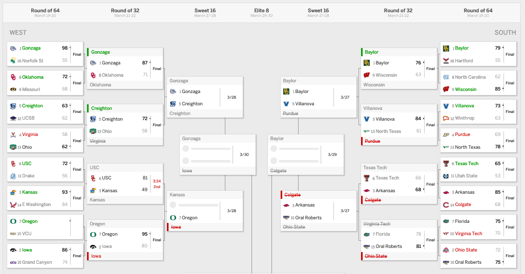
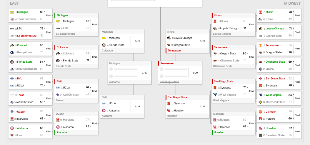
After two rounds, my bracket is better than 38 percent of brackets on ESPN, which puts me in 9.1 millionth place, give or take. I’ve been as low as 10.8 millionth place, so I’ve come up a bit. I still have three of my four Final Four teams and four of eight Elite Eight teams.
When the dust has settled, I’m going to come back and evaluate. Here’s screenshots of my bracket.