What we’re going to cover today:
The R app vs R Studio. One is pointless. One is R Studio.
The R Studio interface generally. Console, Files, Environment and the main work space.
Your first notebook – what happens where.
Creating a project – organizing your files and setting paths automatically.
One last tab: Tutorials.
1. R app vs R Studio
One thing to keep clear in your mind: R is the language, the R app and R Studio are just tools to interact with the language.
The R app is really just a console that will interpret R code. It is mostly useless because of R Studio. However, every semester, I have students start the semester trying to use the R app instead of R Studio. It happens so much I had to make it a meme so they understood clearly.
2. The R Studio Interface
The important parts: The Console, the environment tab and the files tab.
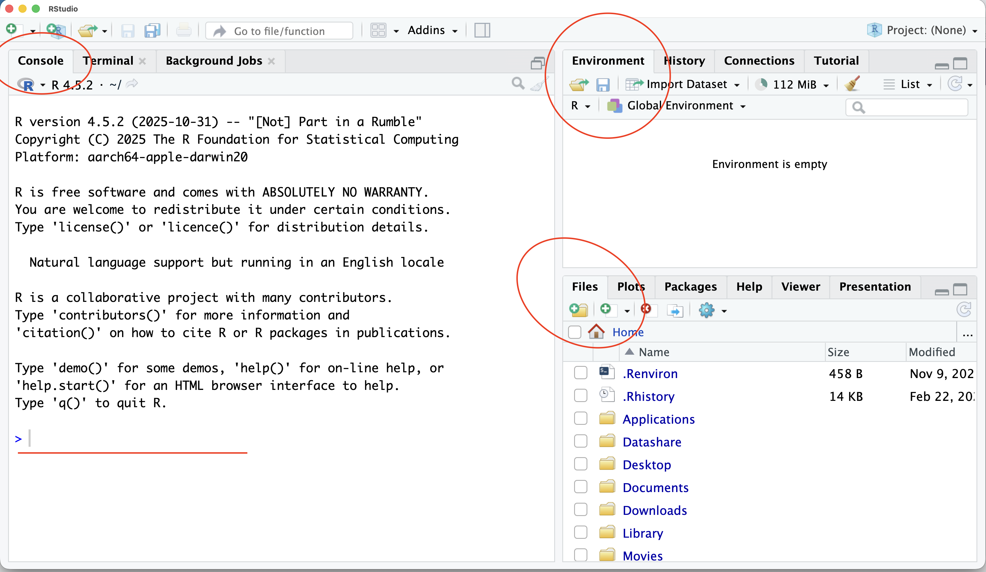
Some R Studio settings to note: Tools > Global Options. You might want to consider turning off all of the auto-saving of things on exit. Personally, I uncheck the first three boxes you can see and set the Save .RData on exit to Never. I want to start with a clean slate every time.
3. Your first notebook
Our first notebook is going to be very simple, but it’s all about seeing the Environment tab in action.
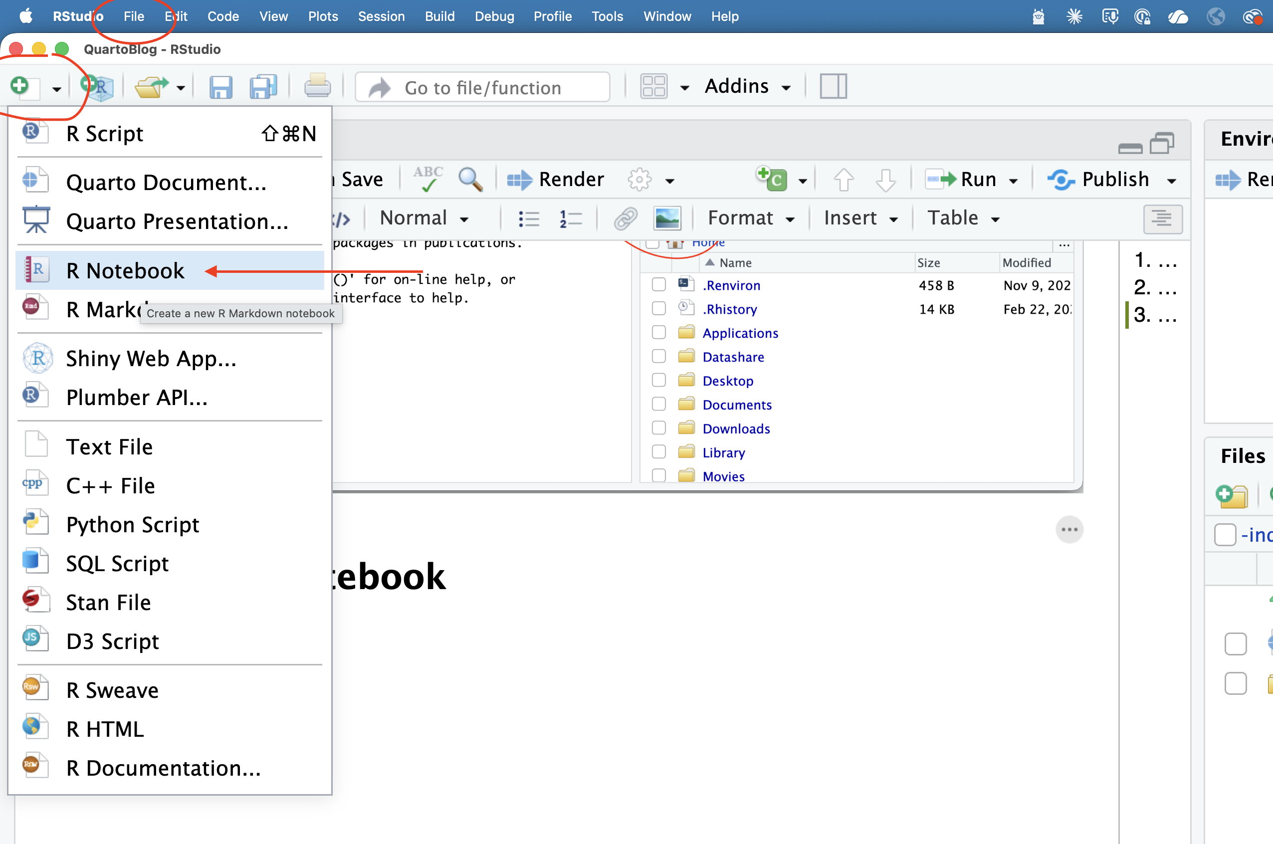
First things first, delete all that auto text. You don’t need it.
Now, write a sentence. Any sentence. A notebook is a markdown file that can also run code. How do you run code? In a code chunk.
See the green C button? Click that and go down to R.
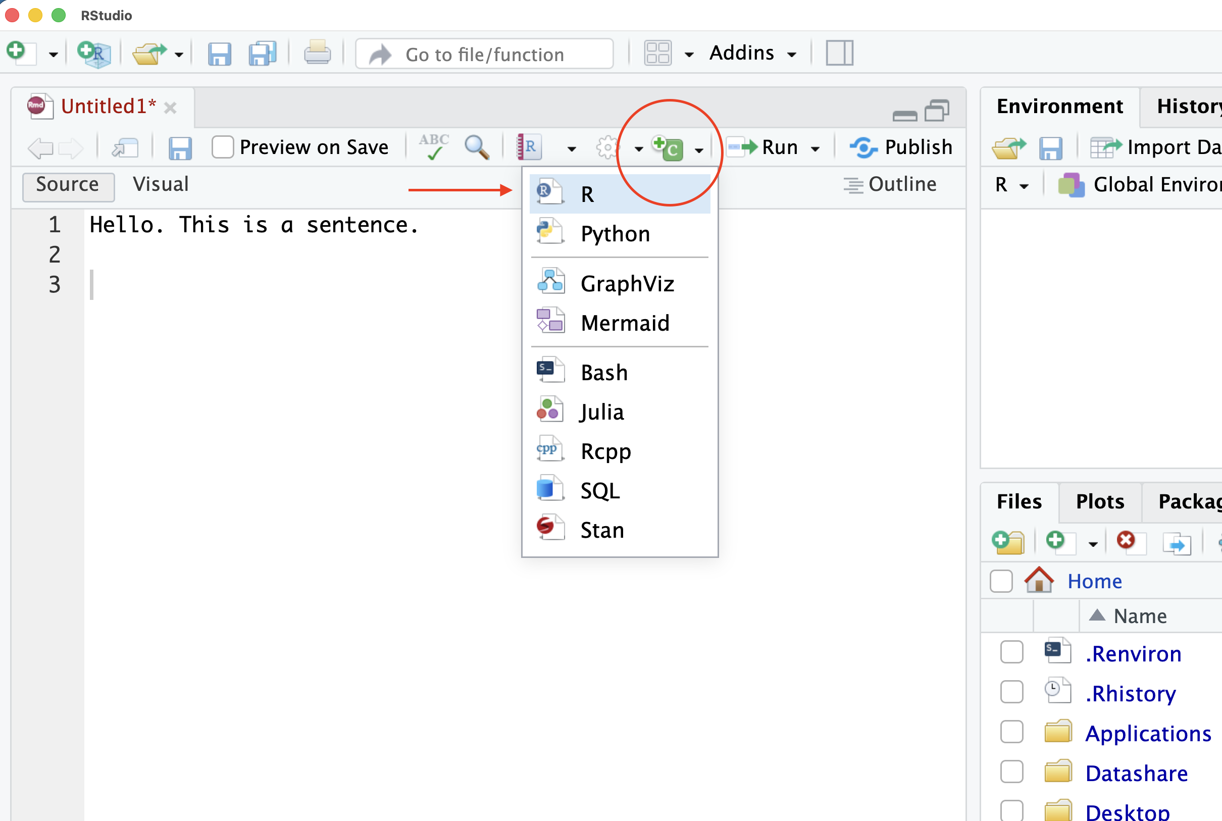
In your code block, simply write 2+2 and click the green triangle on the right side of it to run it.
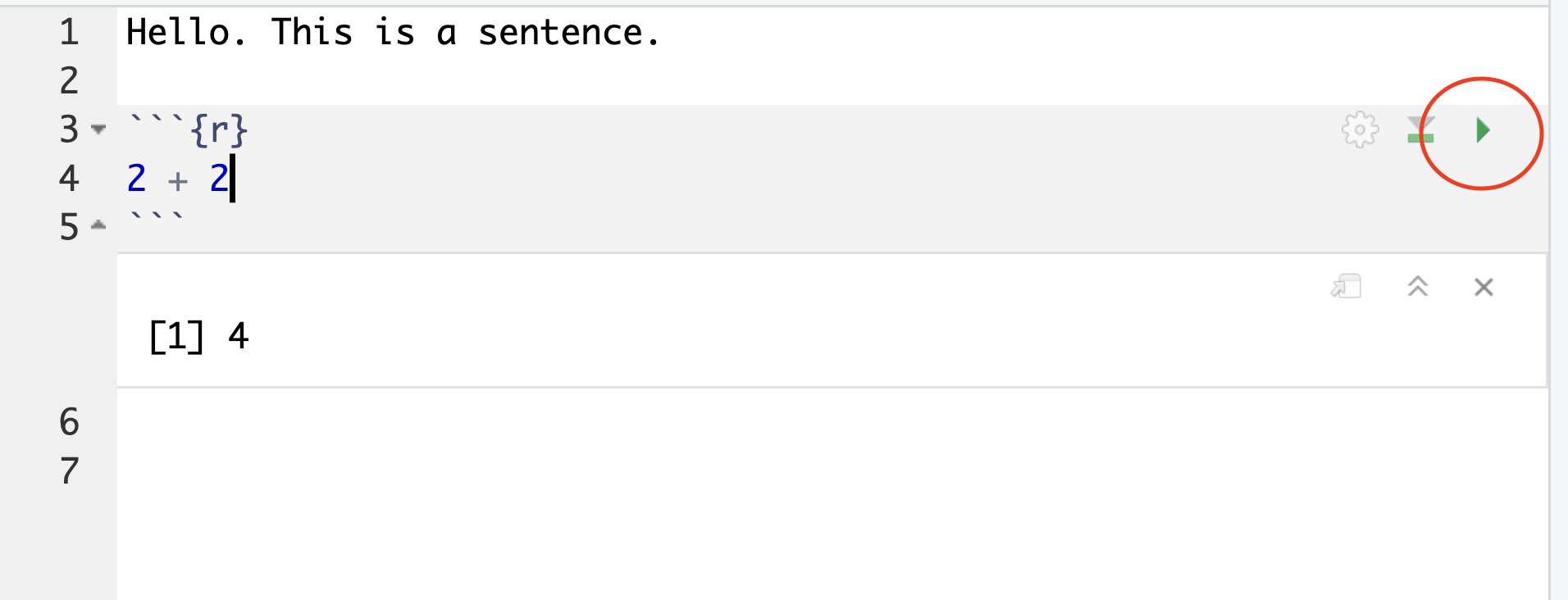
This … is not exciting, but you can run any valid R code in these chunks. Let’s do something meaningful. Replace 2 + 2 with library(tidyverse) and run that. By doing that, you’ve imported 8 very useful libraries that you’re going to use in just about every data analysis.
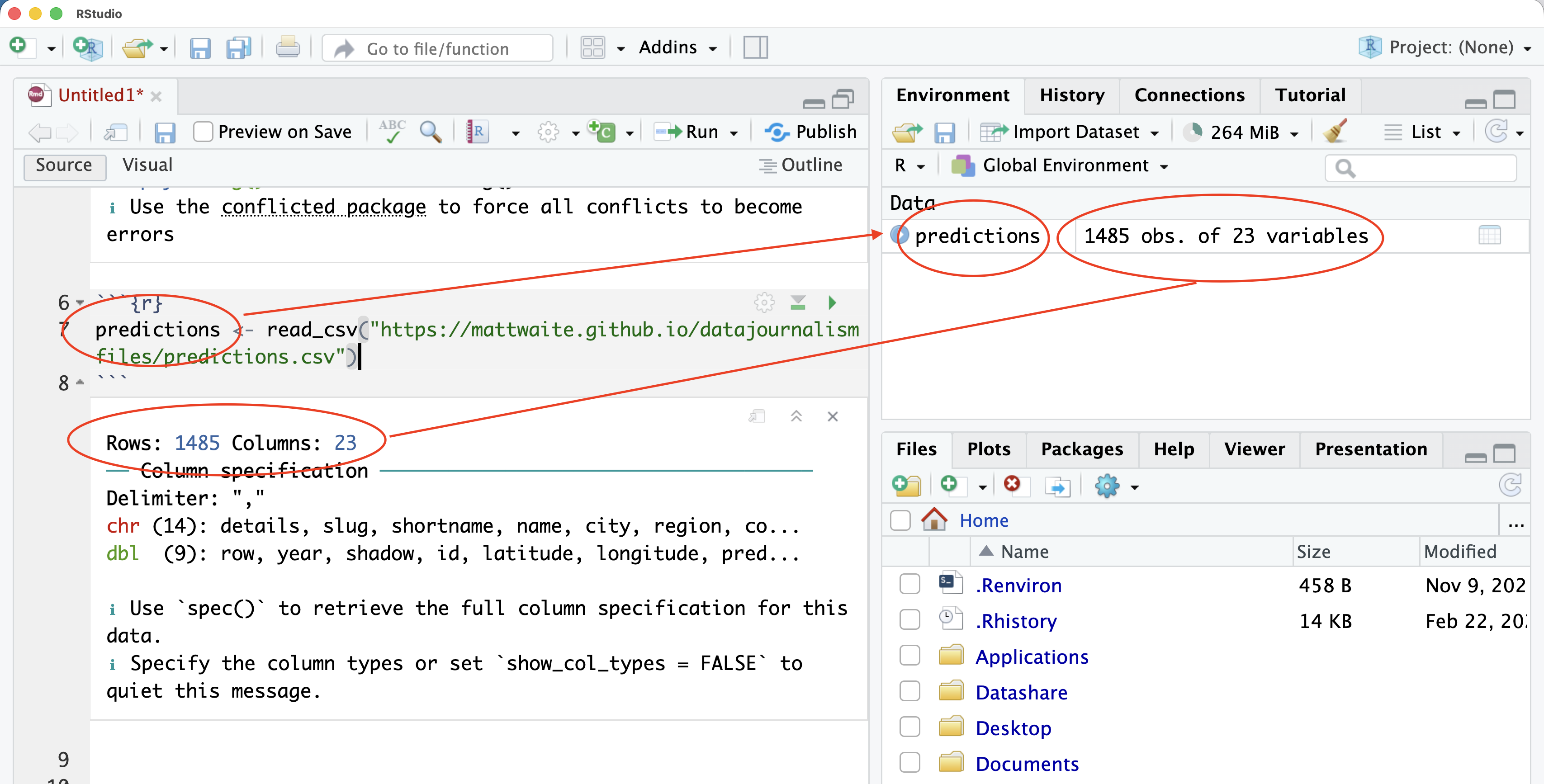
Now, start a new chunk. You can use the green C button again, or you can learn the keyboard shortcut. On a Mac, it’s command-option-i. On Windows, it’s control-alt-i.
In your new code chunk, copy and paste this into it.
predictions <- read_csv("https://mattwaite.github.io/datajournalismfiles/predictions.csv")Now run it.
What did that do? Congrats, you just read in a csv file on my GitHub pages account that has every long winter/early spring prognostication by a groundhog/rodent/lobster/object in North America going back decades. How can you tell? First, the output below the chunk. And then, look in the environment. You’ll see similar things.
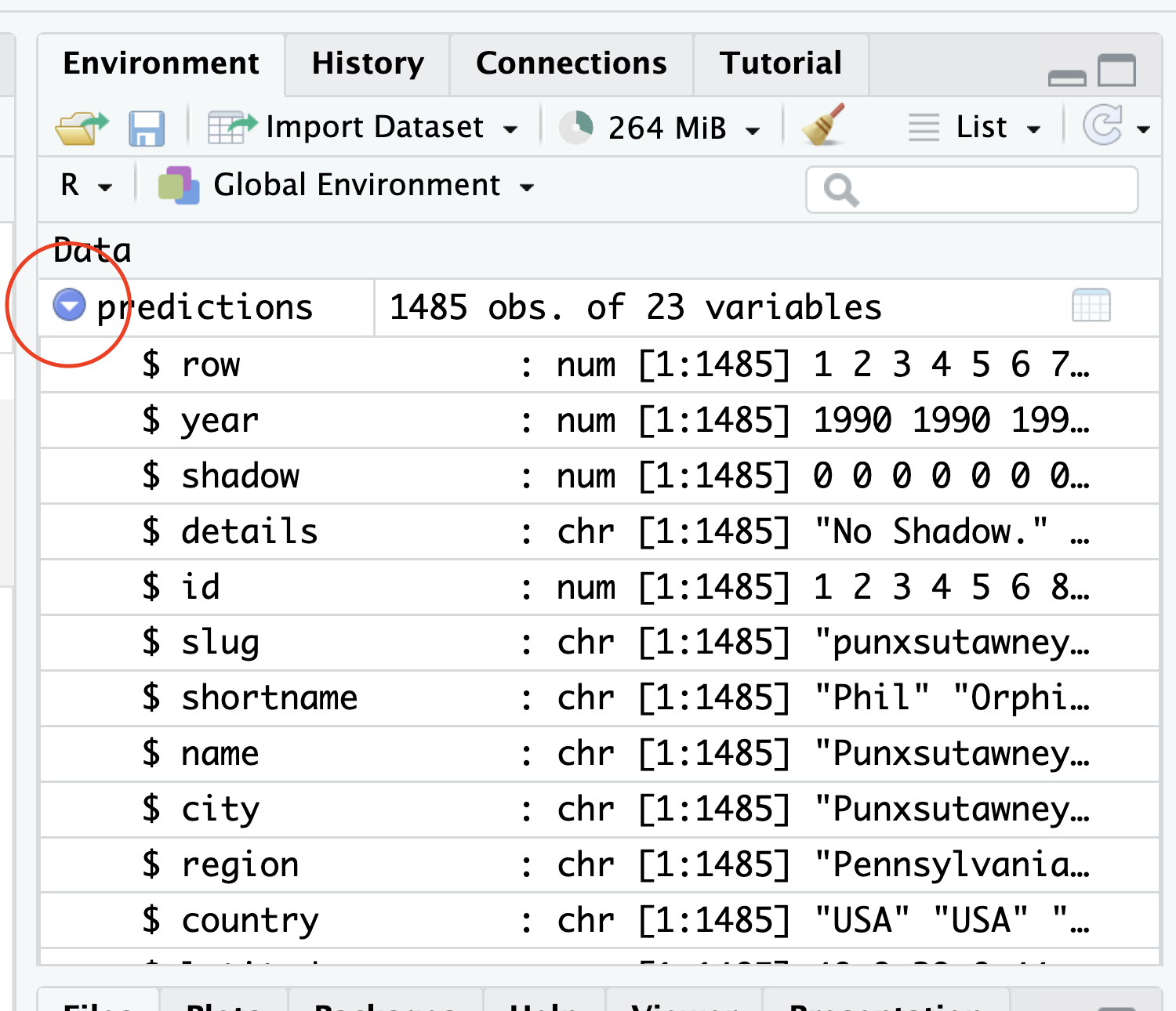
Now, if you click on the blue circle next to predictions in the environment, you’ll get a quick look at the column names contained in the data. This is super useful when you have to do analysis and need to know what column names you have to work with.
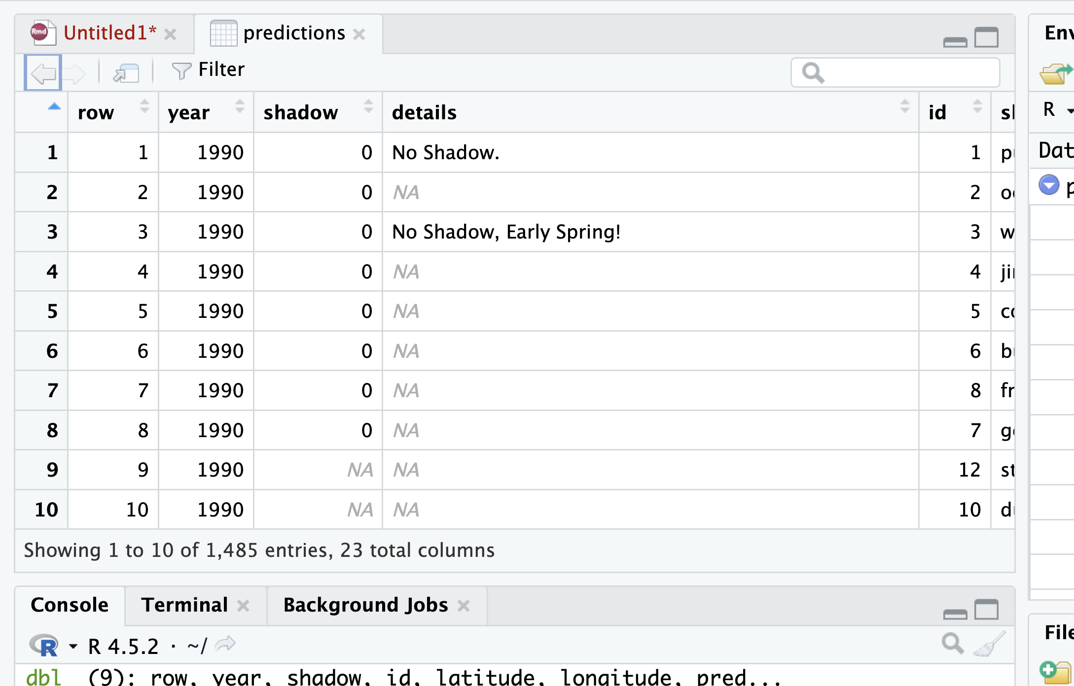
Another view of things is to click on the word predictions and a more spreadsheet like view will pop up.
4. Creating a project to get organized.
Projects are a way to organize your files and your data, while setting directory paths without having to do that yourself. On the upper right corner, you’ll see Project: (None). Click that and go to New Project.
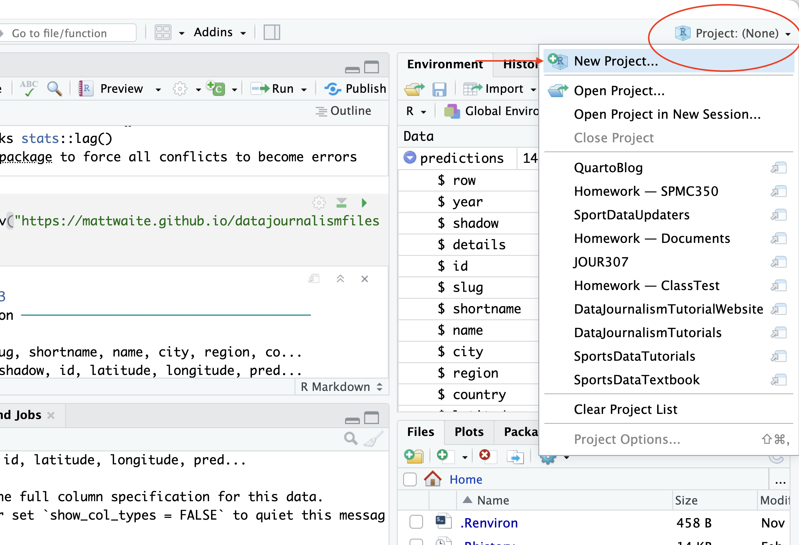
What you do here will depend on your circumstances, but I’m betting this is the first time you’re doing this. As such, we’re going to click New Directory and then New Project.
What comes next: A name and a location. Name your directory Groundhogs because that’s what we’re working with here. Set your file location to something that makes sense (Documents, perhaps).
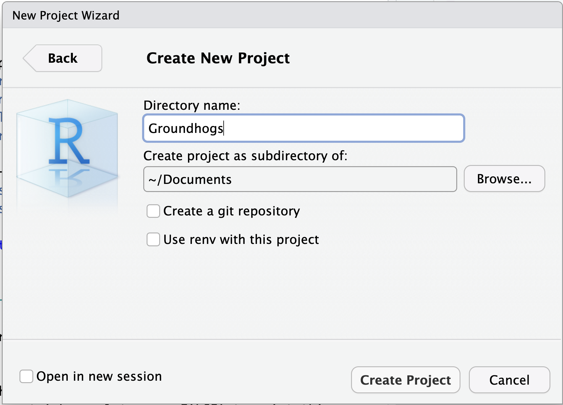
Click create project.
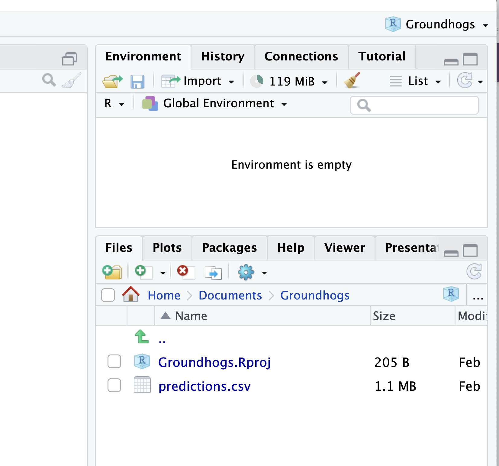
First things first, look at your files tab. Empty now except for an .Rproj file. That Rproj file has very, very little in it and we don’t much care about it.
Let’s put some data into our folder. Download this file and move it into your Groundhog folder.
You may have to refresh it to see it, but once you do move it, this is what it looks like in the files pane.
Now start a new notebook, delete all the text and then save it. See how it automatically wants to save in your project folder?
Add a code chunk to your notebook, type library(tidyverse) in it and run that.
Now, start a new chunk.
Type predictions <- read_csv(" and hit the tab key. See your files pop up? Scroll down to predictions.csv and hit enter.
Run that block.
Now you’ve imported data from your computer, not mine. Nice work.
5. The tutorial pane
If you’re in this class, you’re likely an R beginner. Welcome! We were all there once.
In R, there is a library called learnR that installs interactive tutorials in your R Studio in the Tutorials pane.
I’d call this a commercial but it’s free: I’ve got my whole data journalism class at the University of Nebraska-Lincoln’s College of Journalism and Mass Communications in learnR tutorials. Interested in learning everything from 2+2 to making nearly a dozen different charts all in R? With a different version with local data for all 50 states? For the low low price of nothing?